


Classification of Brain MRI as Tumor/Non Tumor
- Gurucharan M K

- Nov 23, 2020
- 6 min read
Learn to train and apply a simple CNN to differentiate between an MRI with a Tumor and an MRI without one.

Hi everyone! Being a biomedical undergraduate student, wouldn’t it be wrong on my part if I did not show you all an application of AI in Medicine. In this story, I would like to walk-through a real-world application of deep learning to the field of medicine and how it can assist doctors and radiologists to a large extent.
Overview
The dataset I’ll be using for this experiment is obtained from the Kaggle link https://www.kaggle.com/navoneel/brain-mri-images-for-brain-tumor-detection
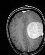
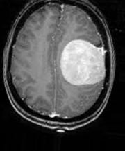
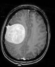
So, first, let me describe the problem that we will be solving over here. In this, we want to classify an MRI Scan of a patient’s brain obtained in the axial plane as whether there is a presence of tumor or not. I am sharing a sample image of what an MRI scan looks like with tumor and without one.


We see that in the first image, to the left side of the brain, there is a tumor formation, whereas in the second image, there is no such formation. So, we can see that there is a clear distinction between the two images. Now how will we use AI or Deep Learning in particular, to classify the images as a tumor or not?
The answer is Convolutional Neural Networks (CNN). CNN or ConvNet is a class of Deep Learning, mostly applied to analyze visual images. There are many frameworks in python to apply CNN such as TensorFlow, PyTorch to train the model. I will be using the Keras library with TensorFlow backend to train this model. Okay! Enough of technical terms, let’s get back to solving the problem.
Step 1: Data Visualization
In the first step, we will analyze the MRI data. In this problem, we have a total of 253 MRI images. Out of them, 155 are labelled “yes”, which indicates that there is a tumor and the remaining 98 are labelled “no”, which indicates that there is no tumor.
print("The number of MRI Images labelled 'yes':",len(os.listdir('yes')))print("The number of MRI Images labelled 'no':",len(os.listdir('no')))The number of MRI Images labelled 'yes': 155The number of MRI Images labelled 'no': 98Now, in a CNN, we have to train a neural network, which can be visualized as a series of algorithms that can recognize the relationships between images in a set of data and can classify them.

In simple terms, a Neural Network functions in the similar way to that of a Human brain. We train the neural network with a set of images with labels (yes or no) and it has the ability to understand the difference between the two classes. Therefore, when we give the neural network a new unlabeled image, it can classify that image with the knowledge acquired during the training process. Simple, isn’t it?
In our example, we have 253 images with 155 belonging to the “yes” class and 98 belonging to the “no” class. We encounter a new problem known as data imbalance. Data imbalance is where the number of observations per class is not equally distributed (here, we have 155 belonging to “yes’ class and only 98 belonging to the “no” class). Wouldn’t our Neural Network not be given enough training in the “no” class? :(
Step 2: Data Augmentation
In order to solve this, we use a technique called Data Augmentation. This is a very important aspect in medicine where there will be many instances of data imbalance. Don’t get it? Come on!, Usually, there would be very less number of unhealthy patients than the number of healthy patients in most cases. Isn’t it?
In Data Augmentation, we take a particular MRI image and perform various sorts of image enhancements such as rotate, mirror and flip to get more number of images. We will apply more augmentation to the class with less number of images to get approximately equal number of images to both classes.
Data Augmentation
From the above images, we can see the various augmentation that has been applied to an MRI image in the “yes” class. In this way, we augment all the images of our dataset.
So after applying Data Augmentation to our dataset, we have 1085 images of “yes” class and 979 images of “no” class. Almost equal, Right?
print(f"Number of examples: {m}")print(f"Percentage of positive examples: {pos_prec}%, number of pos examples: {m_pos}")print(f"Percentage of negative examples: {neg_prec}%, number of neg examples: {m_neg}")Number of examples: 2064 Percentage of positive examples: 52.56782945736434%, number of pos examples: 1085 Percentage of negative examples: 47.43217054263566%, number of neg examples: 979Step 3: Splitting the data
In the next step, we split our data to training set and test set. 80% (1651 images) of the images will go to the training set , which will be used by our neural network to get trained. The remaining 20% (413 images) will go to the test set, with which we will apply our trained neural network and classify them to check the accuracy of our Neural Network.
The number of MRI Images in the training set labelled 'yes':868The number of MRI Images in the test set labelled 'yes':217The number of MRI Images in the training set labelled 'no':783The number of MRI Images in the test set labelled 'no':196Step 4: Building the CNN Model
Okay! Good that you’ve understood so far. Now, where is this Neural Network which I have been telling all this while? It is only in this next step, we design a neural network using Keras library with various convolutional and pooling layers.
model = tf.keras.models.Sequential([tf.keras.layers.Conv2D(16, (3,3), activation='relu', input_shape=(150, 150, 3)),tf.keras.layers.MaxPooling2D(2,2),tf.keras.layers.Conv2D(32, (3,3), activation='relu'),tf.keras.layers.MaxPooling2D(2,2),tf.keras.layers.Conv2D(64, (3,3), activation='relu'),tf.keras.layers.MaxPooling2D(2,2),tf.keras.layers.Flatten(),tf.keras.layers.Dense(512, activation='relu'),tf.keras.layers.Dense(1, activation='sigmoid')])model.compile(optimizer='adam'), loss='binary_crossentropy', metrics=['acc'])The explanation of these layers is a bit complicated for this article. Ill give a explanation of the Neural Network designing in later articles. As of now, you can consider it as a sequence of statements that help in ‘memorizing’ the image data.
Step 5: Pre-Training the CNN model
After this, we will create a “train_generator” and “validation_generator” to store our split images of the training set and the test set into two classes(yes and no).
Found 1651 images belonging to 2 classes.
Found 413 images belonging to 2 classes.
As we see, the 2084 images are split into 1651 (80%) images for the “train_generator” and 413 (20%) images for the “validation_generator”.
Step 6: Training the CNN model
Finally, we come to the stage where we will fit the image data to the trained neural network.
history=model.fit_generator(train_generator,epochs=2,verbose=1,validation_data=validation_generator)
We will train the images data for around 100 “epochs”. An epoch can be thought of an iteration in which we feed the training images again and again for the Neural Network to get trained better with the training images.
Epoch 1/100 50/50 [==============================] - 22s 441ms/step - loss: 0.7400 - acc: 0.5703 - val_loss: 0.6035 - val_acc: 0.6901 Epoch 2/100 50/50 [==============================] - 20s 405ms/step - loss: 0.6231 - acc: 0.6740 - val_loss: 0.5508 - val_acc: 0.7409 Epoch 3/100 50/50 [==============================] - 20s 402ms/step - loss: 0.6253 - acc: 0.6460 - val_loss: 0.5842 - val_acc: 0.6852 Epoch 4/100 50/50 [==============================] - 20s 399ms/step - loss: 0.6421 - acc: 0.6517 - val_loss: 0.5992 - val_acc: 0.6562 Epoch 5/100 50/50 [==============================] - 20s 407ms/step - loss: 0.6518 - acc: 0.6599 - val_loss: 0.5719 - val_acc: 0.7433 Epoch 6/100 50/50 [==============================] - 21s 416ms/step - loss: 0.5928 - acc: 0.6920 - val_loss: 0.4642 - val_acc: 0.8015 Epoch 7/100 50/50 [==============================] - 21s 412ms/step - loss: 0.6008 - acc: 0.6840 - val_loss: 0.5209 - val_acc: 0.7579 Epoch 8/100 50/50 [==============================] - 21s 411ms/step - loss: 0.6435 - acc: 0.6180 - val_loss: 0.6026 - val_acc: 0.6973 Epoch 9/100 50/50 [==============================] - 20s 408ms/step - loss: 0.6365 - acc: 0.6480 - val_loss: 0.5415 - val_acc: 0.7627 Epoch 10/100 50/50 [==============================] - 20s 404ms/step - loss: 0.6383 - acc: 0.6354 - val_loss: 0.5698 - val_acc: 0.7966From the above image, you can see that the “acc” [Accuracy] of the training set keeps improving with each iteration. This means that the Neural Network model is able to improve in classifying the image as Tumor or Not a Tumor. Keep a note of the “val_acc” [Validation Accuracy] which indicates the accuracy of the model on the test_set. Pretty high, Isn’t it?
At the end of the 100th epoch, we see that the trained CNN model has a validation accuracy of 73.85%.
It denotes that our Neural Network can correctly classify about 74% of the test set images as Tumor or Not a Tumor. Good accuracy, ain’t it?
Epoch 100/100 50/50 [==============================] - 20s 402ms/step - loss: 0.3604 - acc: 0.8720 - val_loss: 0.5600 - val_acc: 0.7942Step 7: Analysis of the CNN model
After the training, we finally plot the “accuracy” and “loss” of both “train_generator” and “validation_generator” for all the 100 epochs(iterations).

Coming to the end of this story, using this model, you can feed in an individual MRI image and check whether it has a tumor or not. Cool, isn’t it?
I have shared the link to my GitHub repository where you can find the code and the data for you to try it out. So, go ahead, fork my repository and start experimenting.

Comments